The typical name of file is
a201406220005.fit
Here
a -- type of detector. a is a detector in our single
order spectrograph, c is our echelle.
2014 -- year of exposition
06 -- month
22 -- day
0005 -- order number of the file.
Thus this file was secured in June 22th, 2014, and it was fifth file
that night.
The numbering we change in noon, so we keep the numbering during the night.
We respect the FIT standard.
Raw data FIT header is
COMMENT   FITS (Flexible Image Transport System) format is defined in 'Astronomy
COMMENT   and Astrophysics', volume 376, page 359; bibcode: 2001A&A...376..359H
BZERO   =                32768
BSCALE  =                    1 / REAL=TAPE*BSCALE+BZERO
ORIGIN  = 'PESO    '           / AsU AV CR Ondrejov
OBSERVAT= 'ONDREJOV'           / Name of observatory (IRAF style)
LATITUDE=             49.91056 / Telescope latitude  (degrees), +49:54:38.0
LONGITUD=             14.78361 / Telescope longitud  (degrees), +14:47:01.0
HEIGHT  =                  528 / Height above sea level [m].
TELESCOP= 'ZEISS-2m'           / 2m Ondrejov observatory telescope
TELSYST = 'COUDE   '           / Telescope setup - COUDE or CASSegrain
INSTRUME= 'COUDE700'           / Coude echelle spectrograph
DETECTOR= 'PyLoN 2048x512BX'   / Name of the detector
CHIPID  = 'E2V 42-10 BX'       / Name of CCD chip
BUNIT   = 'ADU     '           / Unit of the array of image data
PREFLASH=                    0 / Length of preflash in seconds
CCDXSIZE=                 2048 / X Size in pixels of digitised frame
CCDYSIZE=                  512 / Y Size in pixels of digitised frame
CCDXPIXE=                 13.5 / Size in microns of the pixels, in X
CCDYPIXE=                 13.5 / Size in microns of the pixels, in Y
DISPAXIS=                    1 / Dispersion axis along lines
GRATNAME= '3       '           / Grating name - ID
SLITTYPE= 'BLADE   '           / Type of slit - blade or image slicers
AUTOGUID= 'NO      '           / Status of autoguider system
SLITWID =                  0.2 / Slit width in mm
COLIMAT = 'open    '           / Collimator mask status
TLE-TRCS= '0       '           / Correction Set
TLE-TRGV= '-11.7 24.7'         / Guiding Value
TLE-TRHD= '10.2101 -9.7519'    / Hour and Declination Axis
TLE-TRRD= '174507.700 -09485'  / Right ascension and Declination
TLE-TRUS= '0.0000 0.0000'      / User Speed
SGH-MCO = 'coude   '           / Mirror Coude Oes
SGH-MSC = 'star    '           / Mirror Star Calibration
SGH-CPA = 'in      '           / Correction plate 700
SGH-CPB = 'out     '           / Correction plate 400
TM-DIFF =                    0 / T1403479375 - P1403479375
OBJECT  = 'HD 161306'          / Title of observation
IMAGETYP= 'object  '           / Type of observation, eg. FLAT
OBSERVER= 'Slechta, Sloup'     / Observers
SYSVER  = 'PESO 835.'
READSPD = '50kHz   '
FILENAME= 'a201406220005.fit'
CAMFOCUS=                5000. / Camera focus position
SPECTEMP=                 21.3 / 17716
SPECFILT=                    1 / Spectral filter
TM_START=                84175 / 23:22:55, 1403479375
UT      = '23:22:55'           / UTC of  start of observation
EPOCH   =                2000. / Same as EQUINOX - for back compat
EQUINOX =                2000. / Equinox of RA and DEC
DATE-OBS= '2014-06-22'         / UTC date start of observation
TM_END  =                 4157 / 01:09:17, 1403485757
EXPTIME =                 6382 / Length of observation excluding pauses
DARKTIME=                 6382 / Length of observation including pauses
CCDTEMP =                 -115 / Detector temperature
EXPVAL  =             0.787732 / Exposure value in photon counts [Mcounts]
BIASSEC = '[1:1,1:512]'        / Overscan portion of frame
TRIMSEC = '[2:2048,140:370]'   / Region to be extracted
GRATANG =                30.25 / 30:15
GRATPOS =                 6457 / Grating angle in increments
DICHMIR =                    2 / Dichroic mirror number
FLATTYPE= 'PROJECT '           / Flat type (Projector/Dome)
COMPLAMP= 'ThAr-BS/15mA'       / Comparison arc setup
RA      = '17:45:07.700'       / 17.752139
DEC     = '-09:48:54.40'       / -9.815111
ST      = '18:26:17'           / Local sidereal time at start of observation
TELFOCUS=                18.69 / Telescope focus (milimeters)
DOMEAZ  =               171.53 / Mean dome azimuth during observation
AIRPRESS=               957.03 / Atmospheric preasure in (hPa)
AIRHUMEX=                75.55 / Air humidity outside the dome
OUTTEMP =                12.36 / Temperature outside of the dome
DOMETEMP=                 15.2 / Temperature inside the dome
GAINM   = 'high    '           / Gain mode
DATE    = '2014-06-23T01:09:36' / file creation date (YYYY-MM-DDThh:mm:ss UT)
CHECKSUM= 'PmAEQm3BPmABPm3B'   / HDU checksum updated 2014-06-23T01:09:36
DATASUM = '1497663368'         / data unit checksum updated 2014-06-23T01:09:36
Reduced (final) data FIT header is
BITPIX  =                    8  /  8-bit ASCII characters
NAXIS   =                    1  /  Number of Image Dimensions
NAXIS1  =                 2047  /  Length of axis
ORIGIN  = 'NOAO-IRAF: WTEXTIMAGE'  /
IRAF-MAX=                   0.  /  Max image pixel (out of date)
IRAF-MIN=                   0.  /  Min image pixel (out of date)
IRAF-B/P=                   32  /  Image bits per pixel
IRAFTYPE= 'REAL FLOATING     '  /  Image datatype
OBJECT  = 'HD 161306         '  /
FILENAME= 'A201406220005.FIT '  /  IRAF filename
FORMAT  = '5G14.7            '  /  Text line format
EXTEND  =                    T / File may contain extensions
ORIGIN  = 'NOAO-IRAF FITS Image Kernel July 2003' / FITS file originator
DATE    = '2014-06-23T18:24:57' / Date FITS file was generated
IRAF-TLM= '2014-06-23T18:25:01' / Time of last modification
OBJECT  = 'HD 161306'          / Name of the object observed
COMMENT   FITS (Flexible Image Transport System) format is defined in 'Astronomy
COMMENT   and Astrophysics', volume 376, page 359; bibcode: 2001A&A...376..359H
OBSERVAT= 'ONDREJOV'           / Name of observatory (IRAF style)
LATITUDE=             49.91056 / Telescope latitude  (degrees), +49:54:38.0
LONGITUD=             14.78361 / Telescope longitud  (degrees), +14:47:01.0
HEIGHT  =                  528 / Height above sea level [m].
TELESCOP= 'ZEISS-2m'           / 2m Ondrejov observatory telescope
TELSYST = 'COUDE   '           / Telescope setup - COUDE or CASSegrain
INSTRUME= 'COUDE700'           / Coude echelle spectrograph
DETECTOR= 'PyLoN 2048x512BX'   / Name of the detector
CHIPID  = 'E2V 42-10 BX'       / Name of CCD chip
BUNIT   = 'ADU     '           / Unit of the array of image data
PREFLASH=                    0 / Length of preflash in seconds
CCDXSIZE=                 2048 / X Size in pixels of digitised frame
CCDYSIZE=                  512 / Y Size in pixels of digitised frame
CCDXPIXE=                 13.5 / Size in microns of the pixels, in X
CCDYPIXE=                 13.5 / Size in microns of the pixels, in Y
GRATNAME= '3       '           / Grating name - ID
SLITTYPE= 'BLADE   '           / Type of slit - blade or image slicers
AUTOGUID= 'NO      '           / Status of autoguider system
SLITWID =                  0.2 / Slit width in mm
COLIMAT = 'open    '           / Collimator mask status
TLE-TRCS= '0       '           / Correction Set
TLE-TRGV= '-11.7 24.7'         / Guiding Value
TLE-TRHD= '10.2101 -9.7519'    / Hour and Declination Axis
TLE-TRRD= '174507.700 -09485'  / Right ascension and Declination
TLE-TRUS= '0.0000 0.0000'      / User Speed
SGH-MCO = 'coude   '           / Mirror Coude Oes
SGH-MSC = 'star    '           / Mirror Star Calibration
SGH-CPA = 'in      '           / Correction plate 700
SGH-CPB = 'out     '           / Correction plate 400
TM-DIFF =                    0 / T1403479375 - P1403479375
IMAGETYP= 'object  '           / Type of observation, eg. FLAT
OBSERVER= 'Slechta, Sloup'     / Observers
SYSVER  = 'PESO 835.'
READSPD = '50kHz   '
FILENAME= 'a201406220005.fit'
CAMFOCUS=                5000. / Camera focus position
SPECTEMP=                 21.3 / 17716
SPECFILT=                    1 / Spectral filter
TM_START=                84175 / 23:22:55, 1403479375
UT      = '23:22:55'           / UTC of  start of observation
EPOCH   =                2000. / Same as EQUINOX - for back compat
EQUINOX =                2000. / Equinox of RA and DEC
DATE-OBS= '2014-06-22'         / UTC date start of observation
TM_END  =                 4157 / 01:09:17, 1403485757
EXPTIME =                 6382 / Length of observation excluding pauses
DARKTIME=                 6382 / Length of observation including pauses
CCDTEMP =                 -115 / Detector temperature
EXPVAL  =             0.787732 / Exposure value in photon counts [Mcounts]
GRATANG =                30.25 / 30:15
GRATPOS =                 6457 / Grating angle in increments
DICHMIR =                    2 / Dichroic mirror number
FLATTYPE= 'PROJECT '           / Flat type (Projector/Dome)
COMPLAMP= 'ThAr-BS/15mA'       / Comparison arc setup
RA      = '17:45:07.700'       / 17.752139
DEC     = '-09:48:54.40'       / -9.815111
ST      = '18:26:17'           / Local sidereal time at start of observation
TELFOCUS=                18.69 / Telescope focus (milimeters)
DOMEAZ  =               171.53 / Mean dome azimuth during observation
AIRPRESS=               957.03 / Atmospheric preasure in (hPa)
AIRHUMEX=                75.55 / Air humidity outside the dome
OUTTEMP =                12.36 / Temperature outside of the dome
DOMETEMP=                 15.2 / Temperature inside the dome
GAINM   = 'high    '           / Gain mode
CHECKSUM= 'PmAEQm3BPmABPm3B'   / HDU checksum updated 2014-06-23T01:09:36
DATASUM = '1497663368'         / data unit checksum updated 2014-06-23T01:09:36
HISTORY = 'Cosmic rays cleaned with dcr program by W. Pych, CAMK & DDO, 2002'
WCSDIM  =                    1 /2
LTM1_1  =                   1.
WAT0_001= 'system=equispec'
WAT1_001= 'wtype=linear label=Wavelength units=angstroms'
TRIM    = 'Jun 23 19:57 Trim data section is [2:2048,140:370]'
ZEROCOR = 'Jun 23 19:57 Zero level correction image is Zero'
FLATCOR = 'Jun 23 19:57 Flat field image is Flat6457.fit with scale=11696.65'
CCDSEC  = '[2:2048,140:370]'
CCDPROC = 'Jun 23 19:57 CCD processing done'
JD      =     2456831.51118056
LJD     =             2456831.
AIRMASS =             2.247607
UTMIDDLE= '0:16:06.0'
BANDID1 = 'spectrum - background fit, weights variance, clean yes'
APNUM1  = '1 1 82.30 146.47'
CTYPE1  = 'LINEAR  '
CRVAL1  =     6262.87451062057
CRPIX1  =                   1.
CDELT1  =    0.230928830906903
CD1_1   =    0.230928830906903
DC-FLAG =                    0 /0
DCLOG1  = 'REFSPEC1 = ca201406220005a201406220004.ms 0.49900547'
DCLOG2  = 'REFSPEC2 = ca201406220005a201406220006.ms 0.50099456'
DISPCOR =                    0
HJD     =     2456831.51685884
VHELIO  =    -2.52434130203828
VLSR    =     12.7800775419465
VSUN    = '   20.    18.    30.  1900.'
END
Explanations:
INSTRUME= 'COUDE700' The coude is equipped with two spectrograph, single order spectrograph and an echelle. The spectrum in the single order spectrograph is depicted to the chip with a Schmidt camera, f=700mm. TLE-TRGV= '-11.7 24.7' The guiding value means offsets. We use a TPOINT model for better guiding. Offsets (saved in the value of keyword TLE-TRGV) are difference between the real and modelled position of the star. The value is in arcseconds. The maximal component is refraction, of course. SGH-MCO = 'coude ' The light beam from the telescope is running directly to he slit header of the single order spectrograph or is reflected by a mirror to the echelle. So this keyword denotes that the mirror is removed from the optical path and the light beam is going to the single order spectrograph. SGH-MSC = 'star ' The configuration for the securing spectra of objects. Alternative: calibration for the securing of flat field or comparison ThAr lamp. SGH-CPA = 'in ' The correction plate of the Schmidt camera is in position IN, it means is IN the optical path. Alternatively it may be removed for another optical configuration of the spectrograph but we do not use this different configurations now. EXPVAL = 0.787732 For the measurement of exposed signal the spectrograph is equipped with exposuremeter. The semi-translucent mirror is put just behing the slit and reflects about 5% of the light to the exposuremeter. The value (counts or kilocounts or Megacounts) denotes the sum of counts. The presented value 0.787732 denotes Mc (Megacounts). The saturation limit depends on the spectral type of the star, the exposuremeter is sensitive in the red color. SPECTEMP= 21.3 The temperature in the coude room (degrees of Celsia) SPECFILT= 1, DICHMIR = 2 We observe in two spectral orders, first (red part of the spectra) and second (blue part of the spectra). The spectrograph is equipped with use dichroic mirrors and color filters for the separation of spectral orders. The dichroic mirror number 2 is standard aluminium layer, filter 1 is a empty hole. It is configuration for the first spectral order. The spectral filter number 5 is for the second spectral order. Another dichroic mirrors (red, blue, infrared) do not improve sensitivity significantly and thus are not used. EPOCH, EQUINOX We use catalogue coordinates with equinox 2000. RA, DEC in fact they are CAT-RA, CAT-DEC. GRATANG, GRATPOS We select spectral ranges with rotating the grating along the vertical axis. The grating angle is measured relatively with respect to the sensor where is a zero point. TELFOCUS The focusing of the telescope is realized by moving the secondary mirror, 0..40mm DOMEAZ Azimuth of the dome. It is not the same as the azimuth of the telescope. The telescope is on the paralactic mounting and thus it is eccentrically with respect to the center of the dome. Thus the telescope is pointing to the dome shutter in different azimuth. BIASSEC = '[1:1,1:512]' The chip has no overscan so we include whole chip to the reduction process. As the keyword should not be empty we define first column as a overscan. TRIMSEC = '[2:2048,140:370]' The part of the chip is covered with callibration light and thus it is to possible to exclude "empty" parts without loss of any data. We exclude the first column and then lower (rows 1 to 140px) and upper (rows 370 to 512px) parts of the chip.
We included our observatory to the database of observatories. In the
path '.../iraf/noao/lib/' there is a file obsdb.dat
where positions of observatories are saved. We included our position
observatory = "ondrejov"
        name = "Ondrejov observatory"
        longitude = 345:12:59
        latitude = 49:54:38
        altitude = 528
        timezone = -1
II.
How to tell the IRAF we use .fit ending instead of .fits?
In the home directory we have to file login.cl. In that file
we use
imtype fit
set imtype="fit"
set imextn="oif:imh fxf:fit,fits..."
In the keyword set imextn must be fit in the first
position.
Example: We use here in Ondrejov
set     imtype          = "fit"
set     imextn          = "oif:imh fxf:fit,fits,at1,spc plf:pl qpf:qp stf:hhh,??h"
III.
imred
ccdred
kpnoslit
onedspec
rv

keep
Here keep is standard ending of file login.cl.
cl < "ccddb$ond/default.cl"
ccdred.instrument = "ccddb$ond/coude.dat"
in the coude.cl and
subset gratposin the coude.dat, respectively.
PACKAGE = imred
   TASK = ccdred

(pixelty=            real real) Output and calculation pixel datatypes
(verbose=                  yes) Print log information to the standard output?
(logfile=              logfile) Text log file
(plotfil=                     ) Log metacode plot file
(backup =                orig/) Backup directory or prefix
(instrum=  ccddb$ond/coude.dat) CCD instrument file
(ssfile =              subsets) Subset translation file
(graphic=             stdgraph) Interactive graphics output device
(cursor =                     ) Graphics cursor input
(version=      2: October 1987)
(mode   =                   ql)
Here we point out backup directory
backup = orig/In the directory where we reduce data we make subdirectory orig. The original raw data will be copied to this backup as (during the reduction process) will be data modified. It will protect us from the necessity to download data again in case of any error in the reduction process.
The command
(instrum= ccddb$ond/coude.dat)will distinguish position of the grating with respect to the increments (keyword GRATPOS in FIT header) which is more sensitive than position denoted in degrees/minutes (see also paragraph IV.).
zerocombine
At first we prepare averaged Zero.
ecl> epar zerocombine

PACKAGE = ccdred
   TASK = zerocombine

   input   =                *.fit  List of zero level images to combine
   (output =                 Zero) Output zero level name
   (combine=              average) Type of combine operation
   (reject =               minmax) Type of rejection
   (ccdtype=                 zero) CCD image type to combine
   (process=                   no) Process images before combining?
   (delete =                   no) Delete input images after combining?
   (clobber=                   no) Clobber existing output image?
   (scale  =                 none) Image scaling
   (statsec=                     ) Image section for computing statistics
   (nlow   =                    0) minmax: Number of low pixels to reject
   (nhigh  =                    1) minmax: Number of high pixels to reject
   (nkeep  =                    1) Minimum to keep (pos) or maximum to reject (neg)
   (mclip  =                  yes) Use median in sigma clipping algorithms?
   (lsigma =                   3.) Lower sigma clipping factor
   (hsigma =                   3.) Upper sigma clipping factor
   (rdnoise=                    7) ccdclip: CCD readout noise (electrons)
   (gain   =                 1.07) ccdclip: CCD gain (electrons/DN)
   (snoise =                   0.) ccdclip: Sensitivity noise (fraction)
   (pclip  =                 -0.5) pclip: Percentile clipping parameter
   (blank  =                   0.) Value if there are no pixels
   (mode   =                   ql)
will average all zerofiles in the directory and save them to Zero.fit:
ecl> zerocombine
List of zero level images to combine (*.fit):

Jul 30 15:04: IMCOMBINE
  combine = average, scale = none, zero = none, weight = none
  reject = minmax, nlow = 0, nhigh = 1
  blank = 0.
                Images     Exp
      a201407170001.fit    1.0
      a201407170002.fit    1.0
      a201407170003.fit    1.0
      a201407170004.fit    2.0
      a201407170005.fit    1.0
      a201407170069.fit    2.0
      a201407170070.fit    2.0
      a201407170071.fit    1.0
      a201407170072.fit    2.0
      a201407170073.fit    2.0

  Output image = Zero, ncombine = 10
ecl>
As one can see, the exposure times do not correspond to expected 0s. The operating software does not enable the premature reading out the CCD chip - when one set exposure time, it is not possible to readout the chip (clouds etc.). However the device enables to control via TTL. So we had to connect an additional electronic element for such additional control. The caused delay is 1-2s for zero and 1s for other files.
flatcombine
Having averaged Zero.fit one can prepare averaged flat field.
PACKAGE = ccdred
   TASK = flatcombine
input   =                *.fit  List of flat field images to combine
(output =                 Flat) Output flat field root name
(combine=              average) Type of combine operation
(reject =            avsigclip) Type of rejection
(ccdtype=                 flat) CCD image type to combine
(process=                  yes) Process images before combining?
(subsets=                  yes) Combine images by subset parameter?
(delete =                   no) Delete input images after combining?
(clobber=                   no) Clobber existing output image?
(scale  =             exposure) Image scaling
(statsec=                     ) Image section for computing statistics
(nlow   =                    1) minmax: Number of low pixels to reject
(nhigh  =                    1) minmax: Number of high pixels to reject
(nkeep  =                    1) Minimum to keep (pos) or maximum to reject (neg)
(mclip  =                  yes) Use median in sigma clipping algorithms?
(lsigma =                   4.) Lower sigma clipping factor
(hsigma =                   4.) Upper sigma clipping factor
(rdnoise=                    7) ccdclip: CCD readout noise (electrons)
(gain   =                 1.07) ccdclip: CCD gain (electrons/DN)
(snoise =                   0.) ccdclip: Sensitivity noise (fraction)
(pclip  =                 -0.5) pclip: Percentile clipping parameter
(blank  =                   1.) Value if there are no pixels
(mode   =                   ql
ecl> flatcombine
List of flat field images to combine (*.fit):
a201407170006.fit: Jul 30 15:06 Trim data section is [2:2048,140:370]
Zero: Jul 30 15:06 Trim data section is [2:2048,140:370]
a201407170006.fit: Jul 30 15:06 Zero level correction image is Zero
a201407170007.fit: Jul 30 15:06 Trim data section is [2:2048,140:370]
a201407170007.fit: Jul 30 15:06 Zero level correction image is Zero
a201407170008.fit: Jul 30 15:06 Trim data section is [2:2048,140:370]
a201407170008.fit: Jul 30 15:06 Zero level correction image is Zero
a201407170009.fit: Jul 30 15:06 Trim data section is [2:2048,140:370]
a201407170009.fit: Jul 30 15:06 Zero level correction image is Zero
a201407170010.fit: Jul 30 15:06 Trim data section is [2:2048,140:370]
a201407170010.fit: Jul 30 15:06 Zero level correction image is Zero
a201407170011.fit: Jul 30 15:06 Trim data section is [2:2048,140:370]
a201407170011.fit: Jul 30 15:06 Zero level correction image is Zero
a201407170054.fit: Jul 30 15:06 Trim data section is [2:2048,140:370]
a201407170054.fit: Jul 30 15:06 Zero level correction image is Zero
a201407170055.fit: Jul 30 15:06 Trim data section is [2:2048,140:370]
a201407170055.fit: Jul 30 15:06 Zero level correction image is Zero
a201407170056.fit: Jul 30 15:06 Trim data section is [2:2048,140:370]
a201407170056.fit: Jul 30 15:06 Zero level correction image is Zero
a201407170057.fit: Jul 30 15:06 Trim data section is [2:2048,140:370]
a201407170057.fit: Jul 30 15:06 Zero level correction image is Zero
a201407170058.fit: Jul 30 15:06 Trim data section is [2:2048,140:370]
a201407170058.fit: Jul 30 15:06 Zero level correction image is Zero

Jul 30 15:06: IMCOMBINE
  combine = average, scale = exposure, zero = none, weight = none
  reject = avsigclip, mclip = yes, nkeep = 1
  lsigma = 4., hsigma = 4.
  blank = 1.
                Images
      a201407170006.fit
      a201407170007.fit
      a201407170008.fit
      a201407170009.fit
      a201407170010.fit
      a201407170011.fit
      a201407170054.fit
      a201407170055.fit
      a201407170056.fit
      a201407170057.fit
      a201407170058.fit

  Output image = Flat6457, ncombine = 11
ecl>
Here the number 6457 in the filename denotes the angle of the grating. As mentioned above, we recognize the flat type with respect to position of the grating in increments better than degrees - it is more accurate.
For reminder (and an example) only:
6457 - around Halpha (first order)
4712 - around Hbeta (second order)
5242 - around Hgamma (second order)
Preparation for doslit task: ccdlist
We prepare list of ThAr spectra and objects. Very convenient is command ccdlist. The convenient format is
ecl> ccdlist ccdtype=comp name+
CCD images to listed (*fit):
a201407170033.fit
a201407170038.fit
where only names of files is depicted. For the comparison see full listing:
ecl> ccdlist ccdtype=comp
CCD images to listed (*fit):
a201407170033.fit[2048,512][ushort][comp][6457]:comp
a201407170038.fit[2048,512][ushort][comp][6457]:comp
The redirection to file will create FILES with lists of ThAr-s and objects:
ccdlist ccdtype=comp name+ > compswill create file comps where will be listed
a201407170033.fit
a201407170038.fit
and
ccdlist ccdtype=object name+ > starswill create file stars where will be listed
a201407170037.fitwhich is star. This is, of course, example. In mentioned files can be a lot of ThAr-s and a lot of objects.
Remark: In that lists must be saved files corresponding to the one depicted spectral region - i.e. we cannot mix Halpha and Hbeta files together.
Task ccdproc
The task ccdproc among others, cuts the uncovered regions of the CCD chip (the flat field covers part of the CCD chip only:

ecl>epar ccdproc

PACKAGE = ccdred
   TASK = ccdproc

images  =                *.fit  List of CCD images to correct
(output =                     ) List of output CCD images
(ccdtype=                     ) CCD image type to correct
(max_cac=                    0) Maximum image caching memory (in Mbytes)
(noproc =                   no) List processing steps only?

(fixpix =                   no) Fix bad CCD lines and columns?
(oversca=                   no) Apply overscan strip correction?
(trim   =                  yes) Trim the image?
(zerocor=                  yes) Apply zero level correction?
(darkcor=                   no) Apply dark count correction?
(flatcor=                  yes) Apply flat field correction?
(illumco=                   no) Apply illumination correction?
(fringec=                   no) Apply fringe correction?
(readcor=                   no) Convert zero level image to readout correction?
(scancor=                   no) Convert flat field image to scan correction?

(readaxi=                 line) Read out axis (column|line)
(fixfile=                     ) File describing the bad lines and columns
(biassec=                image) Overscan strip image section
(trimsec=                image) Trim data section
(zero   =                 Zero) Zero level calibration image
(dark   =                     ) Dark count calibration image
(flat   =                Flat*) Flat field images
(illum  =                     ) Illumination correction images
(fringe =                     ) Fringe correction images
(minrepl=                   1.) Minimum flat field value
(scantyp=            shortscan) Scan type (shortscan|longscan)
(nscan  =                    1) Number of short scan lines

(interac=                  yes) Fit overscan interactively?
(functio=            chebyshev) Fitting function
(order  =                    2) Number of polynomial terms or spline pieces
(sample =                    *) Sample points to fit
(naverag=                    1) Number of sample points to combine
(niterat=                    1) Number of rejection iterations
(low_rej=                   3.) Low sigma rejection factor
(high_re=                   3.) High sigma rejection factor
(grow   =                   0.) Rejection growing radius
(mode   =                   ql)

ecl>ccdproc

List of CCD images to correct (*.fit):
a201407170001.fit: Jul 30 19:04 Trim data section is [2:2048,140:370]
a201407170002.fit: Jul 30 19:04 Trim data section is [2:2048,140:370]
a201407170003.fit: Jul 30 19:04 Trim data section is [2:2048,140:370]
a201407170004.fit: Jul 30 19:04 Trim data section is [2:2048,140:370]
a201407170005.fit: Jul 30 19:04 Trim data section is [2:2048,140:370]
a201407170033.fit: Jul 30 19:04 Trim data section is [2:2048,140:370]
a201407170033.fit: Jul 30 19:04 Zero level correction image is Zero
a201407170033.fit: Jul 30 19:04 Flat field image is Flat6457.fit with scale=11636.81
a201407170037.fit: Jul 30 19:04 Trim data section is [2:2048,140:370]
a201407170037.fit: Jul 30 19:04 Zero level correction image is Zero
a201407170037.fit: Jul 30 19:04 Flat field image is Flat6457.fit with scale=11636.81
a201407170038.fit: Jul 30 19:04 Trim data section is [2:2048,140:370]
a201407170038.fit: Jul 30 19:04 Zero level correction image is Zero
a201407170038.fit: Jul 30 19:04 Flat field image is Flat6457.fit with scale=11636.81
a201407170069.fit: Jul 30 19:04 Trim data section is [2:2048,140:370]
a201407170070.fit: Jul 30 19:04 Trim data section is [2:2048,140:370]
a201407170071.fit: Jul 30 19:04 Trim data section is [2:2048,140:370]
a201407170072.fit: Jul 30 19:04 Trim data section is [2:2048,140:370]
a201407170073.fit: Jul 30 19:04 Trim data section is [2:2048,140:370]
ecl>
Task doslit
ecl> epar doslit


PACKAGE = kpnoslit
   TASK = doslit

objects =               @stars  List of object spectra
(arcs   =               @comps) List of arc spectra
(arctabl=                     ) Arc assignment table (optional)
(standar=                     ) List of standard star spectra

(readnoi=                    0) Read out noise sigma (photons)
(gain   =                 1.07) Photon gain (photons/data number)
(datamax=                INDEF) Max data value / cosmic ray threshold
(width  =                   7.) Width of profiles (pixels)
(crval  =                INDEF) Approximate wavelength
(cdelt  =                INDEF) Approximate dispersion

(dispcor=                  yes) Dispersion correct spectra?
(extcor =                   no) Extinction correct spectra?
(fluxcal=                   no) Flux calibrate spectra?
(resize =                  yes) Automatically resize apertures?
(clean  =                  yes) Detect and replace bad pixels?
(splot  =                  yes) Plot the final spectrum?
(redo   =                  yes) Redo operations if previously done?
(update =                  yes) Update spectra if cal data changes?
(quicklo=                   no) Minimally interactive quick-look?
(batch  =                   no) Extract objects in batch?
(listonl=                   no) List steps but don't process?

(sparams=                     ) Algorithm parameters
(mode   =                   ql)
Now we will jump to the lower level of doslit parameters. We write :e to the line sparams:
(sparams=                     ) Algorithm parameters
(mode   =                   ql)

:e
(we jump to the sparams and start write but the text :e is depicted on the bottom of the window) and thus open the next level:
PACKAGE = kpnoslit
   TASK = sparams

(line   =                INDEF) Default dispersion line
(nsum   =                   10) Number of dispersion lines to sum or median
(extras =                   no) Extract sky, sigma, etc.?

                                -- DEFAULT APERTURE PARAMETERS --
(lower  =                  -4.) Lower aperture limit relative to center
(upper  =                   4.) Upper aperture limit relative to center

                                -- AUTOMATIC APERTURE RESIZING PARAMETERS --
(ylevel =                 0.07) Fraction of peak or intensity for resizing

                                -- TRACE PARAMETERS --
(t_step =                   40) Tracing step
(t_funct=            chebyshev) Trace fitting function
(t_order=                    4) Trace fitting function order
(t_niter=                 1000) Trace rejection iterations
(t_low  =                   3.) Trace lower rejection sigma
(t_high =                   3.) Trace upper rejection sigma

                                -- APERTURE EXTRACTION PARAMETERS --
(weights=             variance) Extraction weights (none|variance)
(pfit   =                fit1d) Profile fitting algorithm (fit1d|fit2d)
(lsigma =                   3.) Lower rejection threshold
(usigma =                   3.) Upper rejection threshold

                                -- BACKGROUND SUBTRACTION PARAMETERS --
(backgro=                  fit) Background to subtract
(b_funct=             legendre) Background function
(b_order=                    1) Background function order
(b_sampl=          -10:-6,6:10) Background sample regions
(b_naver=                   -4) Background average or median
(b_niter=                  400) Background rejection iterations
(b_low  =                   3.) Background lower rejection sigma
(b_high =                   3.) Background upper rejection sigma

                                -- ARC DISPERSION FUNCTION PARAMETERS --
(thresho=                 500.) Minimum line contrast threshold
(coordli=   linelists$thar.dat) Line list
(match  =                   3.) Line list matching limit in Angstroms
(fwidth =                   3.) Arc line widths in pixels
(cradius=                  10.) Centering radius in pixels
(i_funct=            chebyshev) Coordinate function
(i_order=                    4) Order of dispersion function
(i_niter=                 2000) Rejection iterations
(i_low  =                   2.) Lower rejection sigma
(i_high =                   2.) Upper rejection sigma
(refit  =                  yes) Refit coordinate function when reidentifying?
(addfeat=                   no) Add features when reidentifying?

                                -- AUTOMATIC ARC ASSIGNMENT PARAMETERS --
(select =               interp) Selection method for reference spectra
(sort   =                   jd) Sort key
(group  =                  ljd) Group key
(time   =                   no) Is sort key a time?
(timewra=                  17.) Time wrap point for time sorting

                                -- DISPERSION CORRECTION PARAMETERS --
(lineari=                  yes) Linearize (interpolate) spectra?
(log    =                   no) Logarithmic wavelength scale?
(flux   =                  yes) Conserve flux?

                                -- SENSITIVITY CALIBRATION PARAMETERS --
(s_funct=              spline3) Fitting function
(s_order=                    1) Order of sensitivity function
(fnu    =                   no) Create spectra having units of FNU?
(mode   =                   ql)
Run doslit
Now we can start doslit:
ecl> doslit
List of object spectra (@stars):
Edit apertures for a201407170037?  (yes): Y
At first the IRAF will open the graphical window, will depict the cross section of the stellar spectra. We will set the level of signal (bellow our level will be signal recognized as a noise and will be neglected).
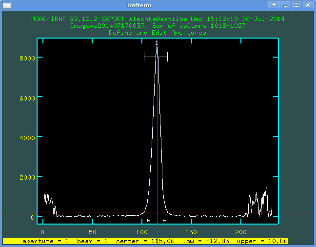
(ylevel = 0.07) Fraction of peak or intensity for resizingupper but we can re-set it manually here. One should put the cursor on asked y-level where signal should be taken into account and press y on the keyboard - the selected y-level will be accounted.
The next step is a background elimination. We press b (the cursor must be inside the graphical window) and IRAF jump depicts the background correction. Selected area can be erased pressing z and defined by s at the beginning and end of better area. It means: we erase "wrong" areas and then put the cursor at the beginning of better area, press s, put the cursor at the end of better area and press s - the better area will be depicted. We standardly mark two areas - one area on each side of the spectra. Then press f (fit) and the background will be denoted and will be subtracted from the spectrum:
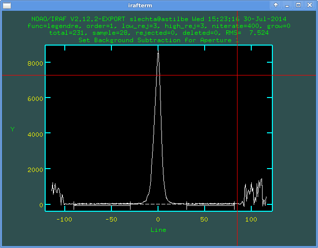
Remark: One should also note that now we use the x-position on the cursor.
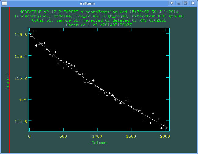
We press q (quit) and jump to the previous level. We can modify again "noise" level, if necessary, press q again and the IRAF will ask us for the tracing the spectrum. We confirm it Y:

Press q and IRAF will switch to the next level, first manual identification of ThAR lines for the first approximation of the dispersion function.
We mark selected line m (mark) and of course may it also erase, d (delete) when we mistakenly mark wrong line. The IRAF will ask for the wavelength (it is good to write the wavelength up to the first decimal place):
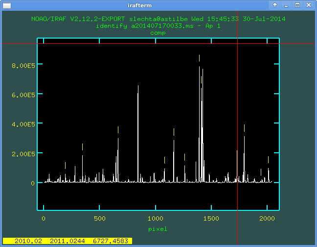

Then press f (fit) and first iteration of dispersion function is
found:
Linear part:
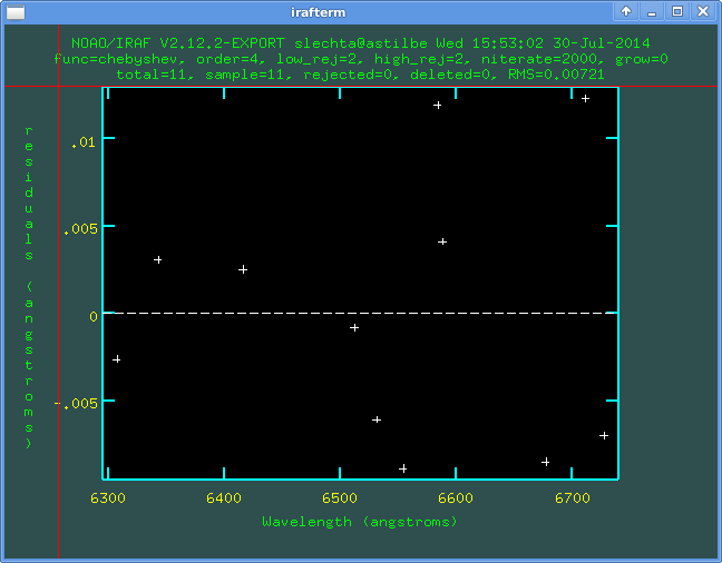
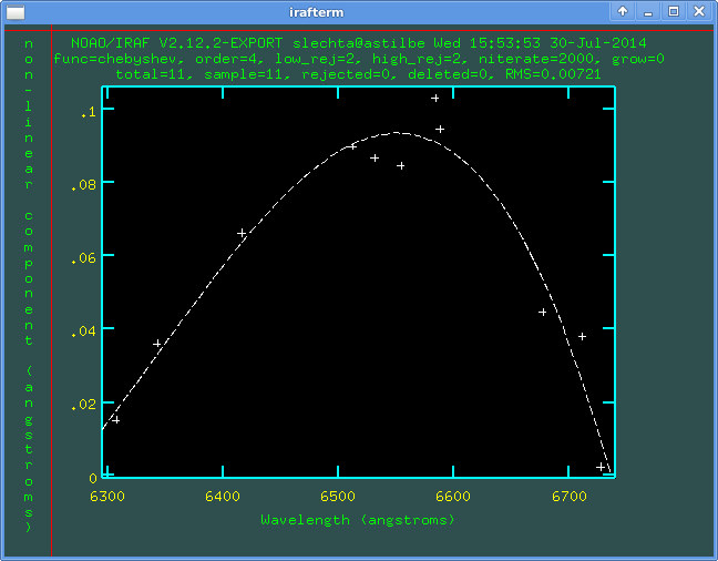
For example we offer usually used lines being identified for Halpha region here in Ondrejov:

Having this one can switch to the environment where lines are identified and press q. Thus it leave the graphical window (back to the command line) and defined it is NOT necessary to redefine coordinate system and confirm YES for automatic identification of lines.
Extract arc reference image a201407170033
Determine dispersion solution for a201407170033
a201407170033.ms.fit: w1 = 6263.483670280945, w2 = 6735.988208287622, dw = 0.230940634411865, nw = 2047
  Change wavelength coordinate assignments? (yes|no|NO): N
Extract object spectrum a201407170037
Assign arc spectra for a201407170037
Extract and reidentify arc spectrum a201407170033
a201407170037a201407170033.ms - Ap 1 17/17   15/17   -3.72E-4    -8.61E-5  -1.4E-8  0.00586
Fit dispersion function interactively? (no|yes|NO|YES) (yes): Y
it will switch back to the graphical window with ThAr lines, one can press l (lines) and a lot of lines will be found.
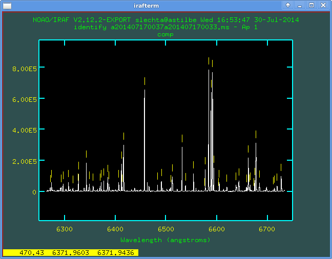
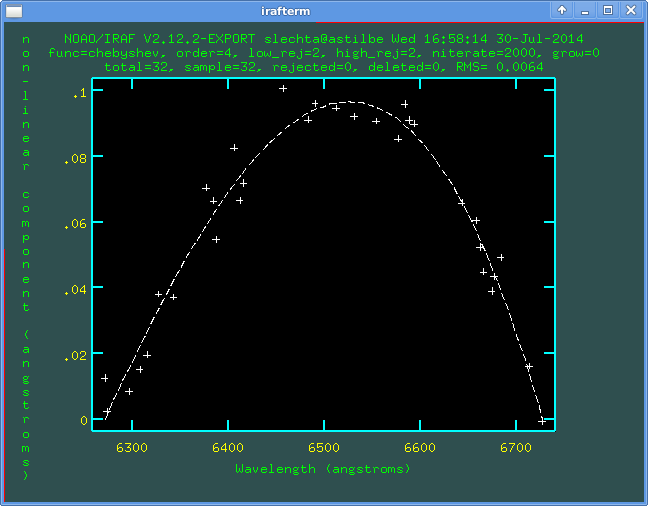
We point out important parameters: number of identified lines and rms error. Of course, it depends on spectrographs. Here in Ondrejov we have limit (usually) rms 0.008 or 0.004 (in the first and second spectral orders, respectively) and number of lines should be over 28-29.
This is idenfitication of ThAr lines on the first spectrum in the list comps. Press q when we are satisfied with the identification and switch to the second ThAr spectrum where we repeat automatic identification process. Thus we obtain two ThAr spectra, one exposed before the star and one exposed after the star. Having this, press q and we jump out of the graphical windown and the IRAF will ask about depiction of stellar spectra:
Extract and reidentify arc spectrum a201407170038
Dispersion correct a201407170037
a201407170037.ms.fit:
Splot spectrum? (no|yes|NO|YES): Y
and we will have final reduced spectrum:
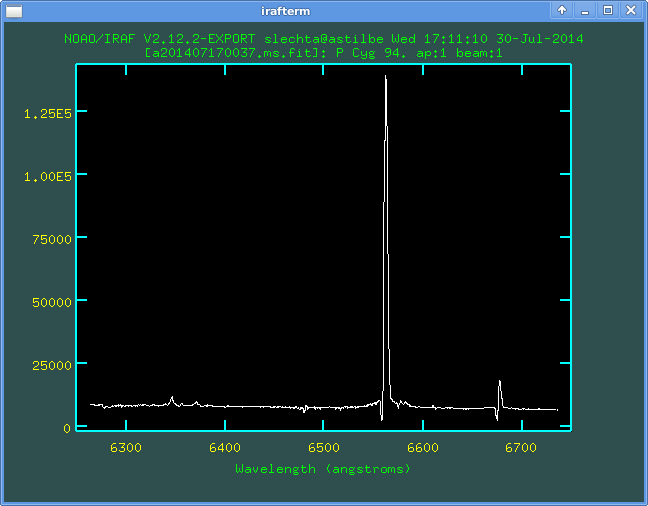
Remark 1: one can see distinguishing of different types of reduced/non-reduced stellar spectra. Original name was a201407170037.fit, calibrated to wavelengths is a201407170037.ms.fit
Remark 2: The ending *ms.fit also is on the first ThAr spectrum in the list comps. It is just the ThAr spectrum we manually identified spectral lines.
Heliocentric correction
The keyword rvcorrect computes the value of the heliocentric correction and writes it to the FIT header.
ecl>epar rvcorrect

PACKAGE = rv
   TASK = rvcorrect

(files  =                     ) List of files containing observation data
(images =             *.ms.fit) List of images containing observation data
(header =                  yes) Print header?
(input  =                  yes) Print input data?
(imupdat=                  yes) Update image header with corrections?

(epoch  =                INDEF) Epoch of observation coordinates (years)
(observa=             ondrejov) Observatory
(vsun   =                  20.) Solar velocity (km/s)
(ra_vsun=                  18.) Right ascension of solar velocity (hours)
(dec_vsu=                  30.) Declination of solar velocity (degrees)
(epoch_v=                1900.) Epoch of solar coordinates (years)

(year   =                     ) Year of observation
(month  =                     ) Month of observation (1-12)
(day    =                     ) Day of observation
(ut     =                     ) UT of observation (hours)
(ra     =                     ) Right ascension of observation (hours)
(dec    =                     ) Declination of observation (degrees)
(vobs   =                   0.) Observed radial velocity
(hjd    =                     ) Helocentric Julian Day (output)
(vhelio =                     ) Helocentric radial velocity (km/s) (output)
(vlsr   =                     ) Local standard or rest radial velocity (km/s) (o
(mode   =                   ql)
while commant dopcor will shift the spectrum.
ecl>epar dopcor

PACKAGE = onedspec
   TASK = dopcor

input   =             *.ms.fit  List of input spectra
output  = *%.ms.fit%hc.ms.fit%  List of output spectra
redshift=              -vhelio  Redshift or velocity (Km/s)
(isveloc=                  yes) Is the redshift parameter a velocity?
(add    =                   no) Add to previous dispersion correction?
(dispers=                  yes) Apply dispersion correction?
(flux   =                   no) Apply flux correction?
(factor =                   3.) Flux correction factor (power of 1+z)
(apertur=                     ) List of apertures to correct
(verbose=                   no) Print corrections performed?
(mode   =                   ql)
Running this commands:
ecl> rvcor
# RVCORRECT: Observatory parameters for Ondrejov observatory
#       latitude = 49:54:38
#       longitude = 345:12:59
#       altitude = 528
##YR MO DY    UT       RA       DEC       VOBS
##   HJD          VOBS   VHELIO     VLSR   VDIURNAL   VLUNAR  VANNUAL   VSOLAR
2014  7 17 21:10:18 20:17:47  38:01:58      0.0
2456856.38512     0.00     7.58    25.12      0.141    0.006    7.432   17.540
ecl>
ecl>dopcor
List of input spectra (*.ms.fit):
List of output spectra (*%.ms.fit%hc.ms.fit%):
Redshift or velocity (Km/s) (-vhelio):
ecl>
Remark 1: The commands rvcorrect and dopcor are trying to work with all files *ms.fit - it means also the first ThAr file. However we do not write position of the telescope or position of stars to the FIT header of ThAr-s (right ascension, declination) and thus it is not possible to find heliocentric correction for ThAr-s. IRAF therefore writes warnings:
ecl> rvcor
# RVCORRECT: Observatory parameters for Ondrejov observatory
#       latitude = 49:54:38
#       longitude = 345:12:59
#       altitude = 528
Warning: Image header parameter not found (UTMIDDLE)
##YR MO DY    UT       RA       DEC       VOBS
##   HJD          VOBS   VHELIO     VLSR   VDIURNAL   VLUNAR  VANNUAL   VSOLAR
2014  7 17 21:10:18 20:17:47  38:01:58      0.0
2456856.38512     0.00     7.58    25.12      0.141    0.006    7.432   17.540
ecl>
ecl>dopcor

List of input spectra (*.ms.fit):
List of output spectra (*%.ms.fit%hc.ms.fit%):
Redshift or velocity (Km/s) (-vhelio):
Warning: Image header parameter not found (vhelio)
ecl>
It is not dangerous for reduction process nevertheless we recommend to copy stellar spectra to special subdirectory (for example NONHC or something similar) and rvcor and dopcor there.
Remark 2: Note that heliocentric correction shifted spectrum is
renamed to
a201407170037hc.ms.fit so we have three types of stellar spectra:
a201407170037.fit - original
a201407170037.ms.fit - wavelength calibrated
a201407170037hc.ms.fit- wavelength calibrated + heliocentric
calibration shifted
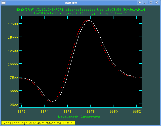
Remark 3: The value of heliocentric correction is (in this example) +7.579km/s One can see that spectra are indeed shifted (the picture is detailed to helium line 6678):
